
Detecting When Things Change: Bayesian Change Point Analysis

Suppose you’re looking at count data over time: disasters per year, trades per hour, defaults per month. You suspect the rate changed at some point, but you don’t know when. How do you find the change point and quantify your uncertainty?
This is a classic problem in Bayesian statistics. We’ll walk through it using the UK Coal Mining Disasters dataset (1851-1962), which records the number of major mining disasters per year. The data shows a clear drop in disaster frequency, but when exactly did it happen?
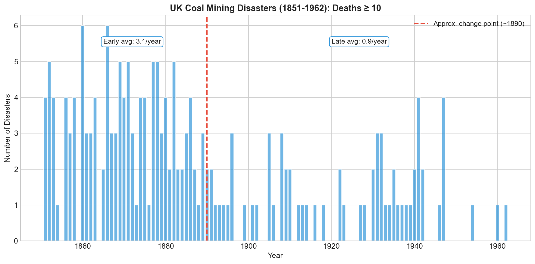
The early years average around 3 disasters per year. The later years average closer to 1. Somewhere in between, something changed. We want to find that transition point. Naruraly in the data above we can see that but how can we be more scientific about it?
The Historical Context
Coal mining in 19th century Britain was brutal. Before regulation, mines were death traps. Children as young as five worked underground. Explosions, collapses, and gas poisonings were routine.
Reform came in waves. The Mines and Collieries Act of 1842 banned women and children under 10 from underground work. The Coal Mines Regulation Act of 1860 raised the minimum age to 12 and introduced basic safety rules. But the real turning point came with the Coal Mines Regulation Act of 1872, which required certified mine managers, mandated proper ventilation, and assigned clear legal responsibility for safety to mine owners.
Further amendments in 1887 tightened enforcement. By the 1890s, the cumulative effect of decades of legislation, union pressure, and government inspection had fundamentally changed how mines operated.
Our model should find this. If the data reflects reality, we’d expect the change point to land somewhere in the 1880s or 1890s, after the major reforms had time to take effect.
The Poisson Distribution (For Counting Events)
When you’re counting events in a fixed period, the Poisson distribution is the standard model. It has one parameter: λ (lambda), the average rate.
P(k events) = λᵏ × e⁻λ / k!
Where:
λ = average rate of events
k = number of events (0, 1, 2, ...)
If λ = 3, you expect about 3 events per period. The distribution tells you the probability of seeing 0, 1, 2, 3, ... events.
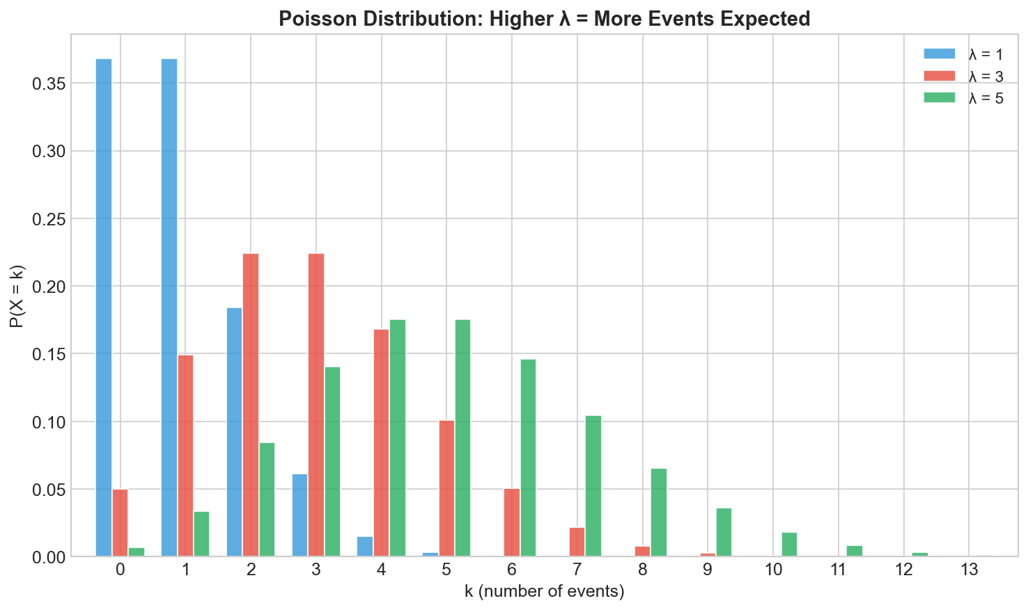
Higher λ shifts probability toward larger counts. With λ = 1, seeing 5 events is rare. With λ = 5, seeing 5 events is common.
The Change Point Model
We believe the disaster rate changed at some unknown year τ (tau). Before τ, disasters follow Poisson(λ₁). After τ, they follow Poisson(λ₂).
Three unknowns:
λ₁ = disaster rate in the early period
λ₂ = disaster rate in the late period
τ = the year when the rate changed
Our goal is to estimate all three.
What Are Priors?
In Bayesian statistics, we specify what we believe about each parameter before seeing the data. This is called a prior distribution.
Think of it as answering: “If I hadn’t looked at the data yet, what values would I consider plausible?”
For τ (the change point): We have no idea which year the change occurred. Any year is equally likely. So we use a Uniform prior.
τ ~ Uniform(1851, 1962)
Every year gets equal probability: 1/112.
For λ₁ and λ₂ (the rates): We know they must be positive (can’t have negative disasters). We think smaller rates are more plausible than huge ones, but we’re not very opinionated. So we use an Exponential prior.
λ₁ ~ Exponential(mean ≈ 1.7) λ₂ ~ Exponential(mean ≈ 1.7)
Poisson vs Exponential: Two Different Roles
This is where things get confusing. Both distributions involve λ. But they serve completely different purposes.
The Poisson distribution models the actual disaster counts. Given a rate λ, it tells you the probability of observing 0, 1, 2, ... disasters.
The Exponential distribution is our prior belief about λ itself. Before seeing data, we think λ is probably somewhere between 0 and 5, with smaller values more likely than larger ones.
Poisson = “How many disasters happen given rate λ?” Exponential = “What rates λ do we think are plausible before seeing data?”
The Exponential is not claiming disasters follow an exponential process. It’s just a way to express uncertainty about the rate parameter.
How the Model Finds the Answer
The model tests thousands of (τ, λ₁, λ₂) combinations. Combinations with high likelihood get kept more often. Combinations with low likelihood get rejected.
After sampling:
τ clusters around 1890
λ₁ clusters around 3.1 disasters/year
λ₂ clusters around 0.9 disasters/year
The prior for τ was Uniform (all years equally likely). The posterior for τ is concentrated around 1890. The data transformed our belief.
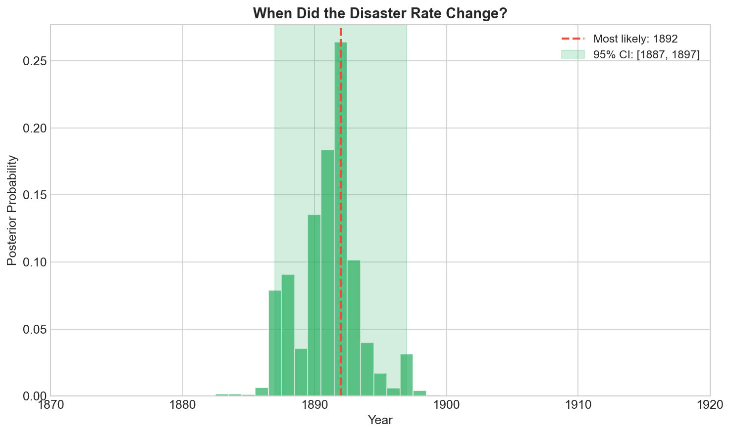
The posterior shows high probability mass around 1889-1891. This is our best estimate for when the change occurred, with uncertainty quantified.
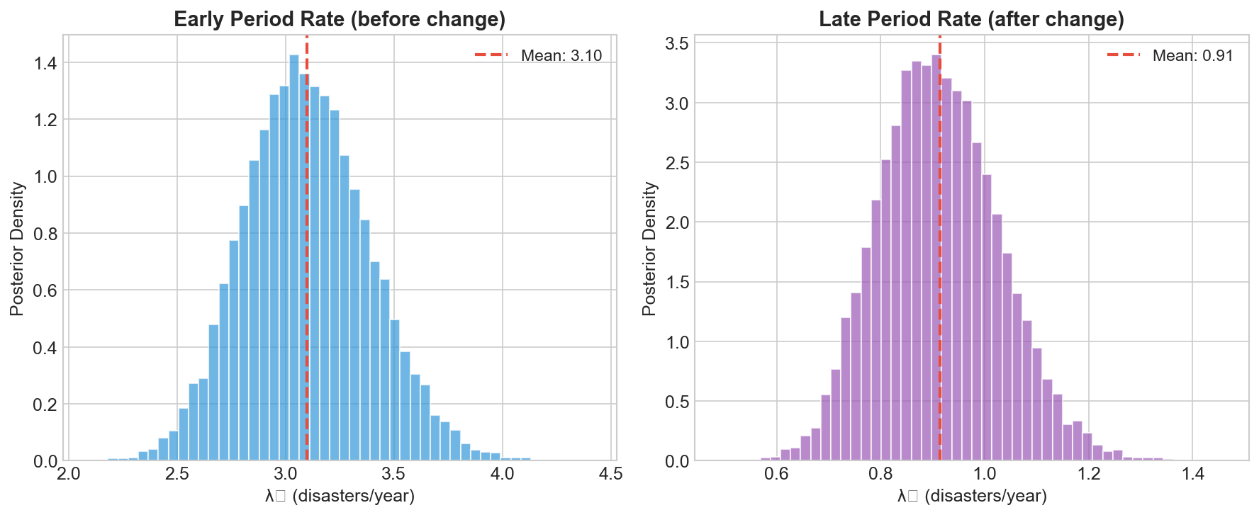
The two rate distributions are well separated. The early period had about 3 disasters per year. The late period had about 1. Strong evidence that a real change occurred.
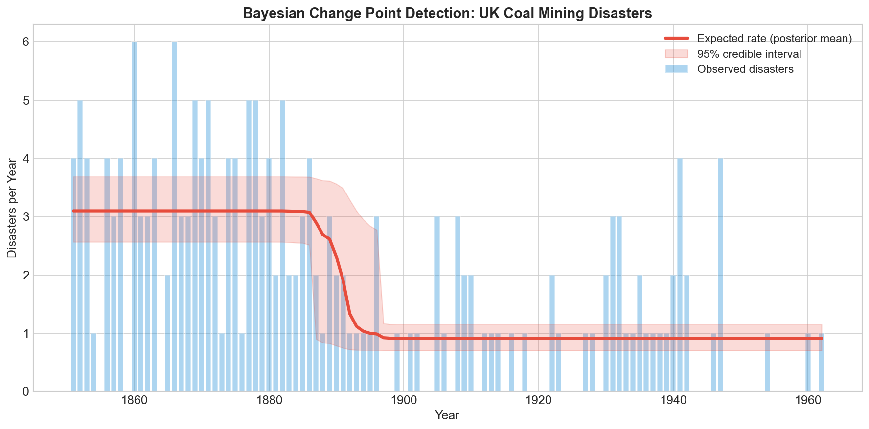
The expected rate shows a clear transition. The uncertainty band captures when the switch happened.
Limitations
This model assumes exactly one change point. The data might actually have:
No change point (constant rate)
Two or more change points
A gradual transition rather than an abrupt switch
You could extend the model to handle multiple change points, or use model comparison techniques to decide which structure fits best. For this dataset, one change point seems reasonable based on visual inspection and historical context.
Summary
The Bayesian change point model lets you:
Estimate when a rate changed (τ)
Estimate the rates before and after (λ₁, λ₂)
Quantify uncertainty in all estimates
The Poisson distribution models count data. The Exponential distribution expresses prior uncertainty about the rate. Bayes’ theorem combines prior beliefs with observed data to produce the posterior.
For the coal mining data, the model finds a change around 1890, with the disaster rate dropping from about 3 per year to about 1. This aligns with the historical record: the Coal Mines Regulation Acts of 1872 and 1887 had fundamentally transformed the industry by this point. The model, knowing nothing about Victorian politics, independently arrives at the same conclusion historians would.