
Portfolio Optimization Basics

You have $100,000 to invest across six ETFs. How do you split it?
You could go equal weight. Put $16,667 in each and call it a day. But that ignores everything we know about these assets. Some have higher expected returns. Some are less volatile. Some zig when others zag. Why not use that information?
That’s what portfolio optimization does. You feed it historical returns, and it spits out weights that balance return against risk. We’ll look at Mean-Variance optimization which aims to balance the returns and risk of a portfolio, and its sister, MVSK, which accounts for futher moments of skewness and kurtosis.
The Assets
We’re using six sector ETFs:
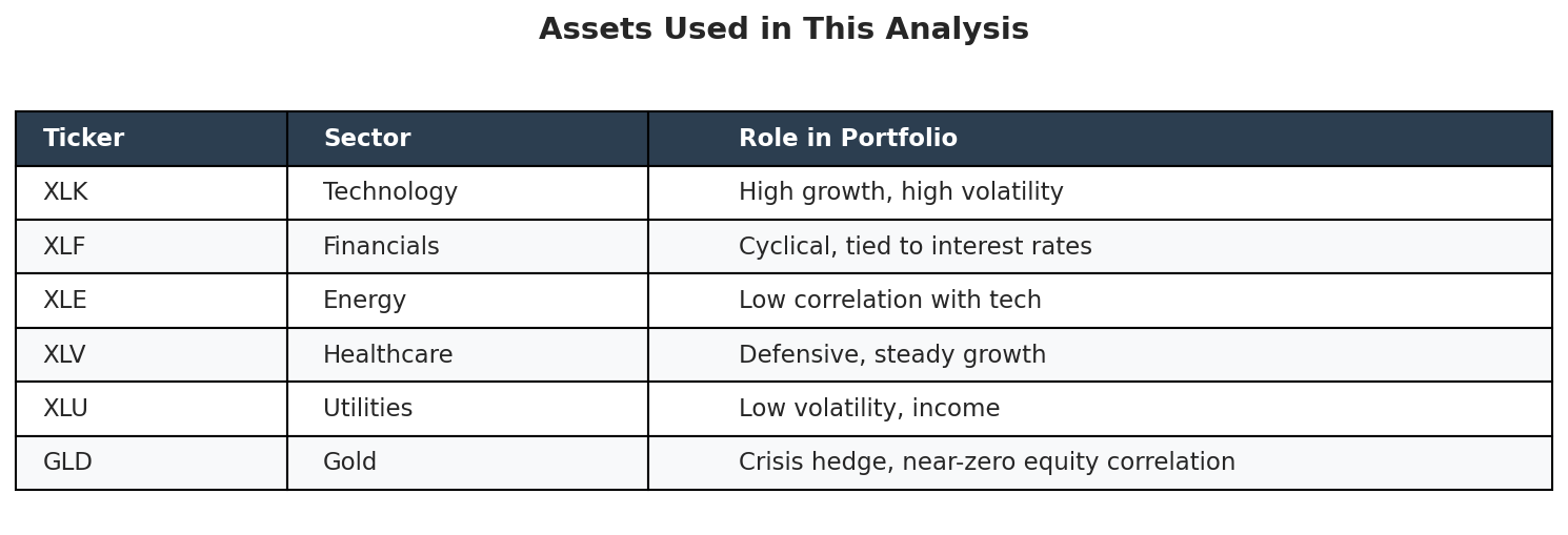
The data covers 2018 to 2024.
Correlations Matter
Before optimizing, look at how these assets move together.
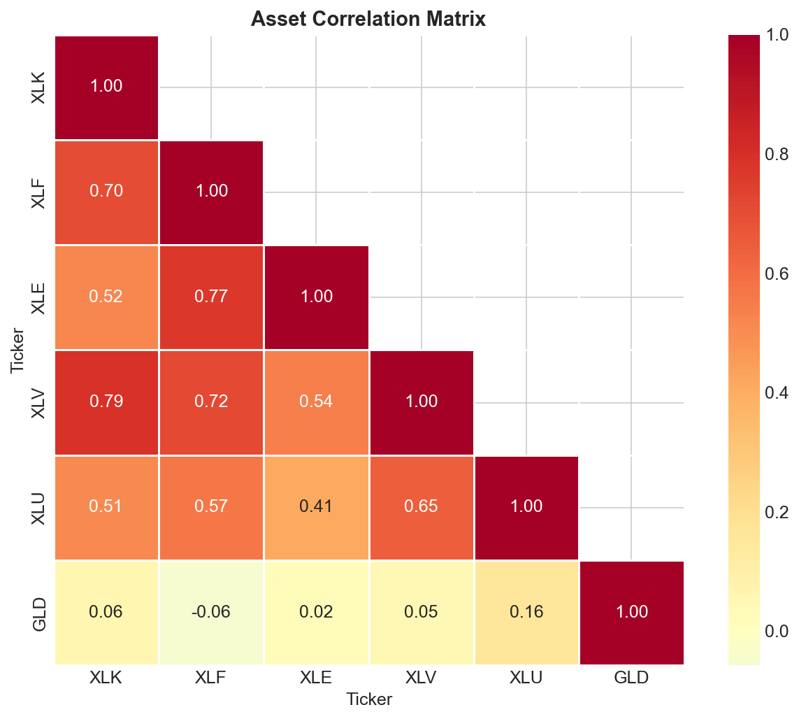
A correlation of 1.0 means two assets move in lockstep. No diversification benefit there. Correlation near zero means they move independently. Negative correlation means they tend to move opposite directions.
GLD (Gold) has near-zero correlations with the equity ETFs. When stocks tank, gold often holds steady or goes up. That makes it useful even if its returns are nothing special on their own.
XLE (Energy) also marches to its own beat. Oil prices respond to supply shocks and geopolitics more than general market sentiment.
Mean-Variance Optimization
MV optimization maximizes a utility function that rewards returns and penalizes variance:
U = μ - (λ/2)σ²
Where:
μ is the portfolio’s expected return (annualized)
σ² is the portfolio’s variance (how much returns bounce around)
λ is your risk aversion. Higher values mean you hate volatility more.
Think of λ as a dial. Set it to 1 and the optimizer goes aggressive, chasing returns. Set it to 10 and it gets conservative, prioritizing stability. A value around 3 is moderate.
With λ = 3, here’s what comes out:
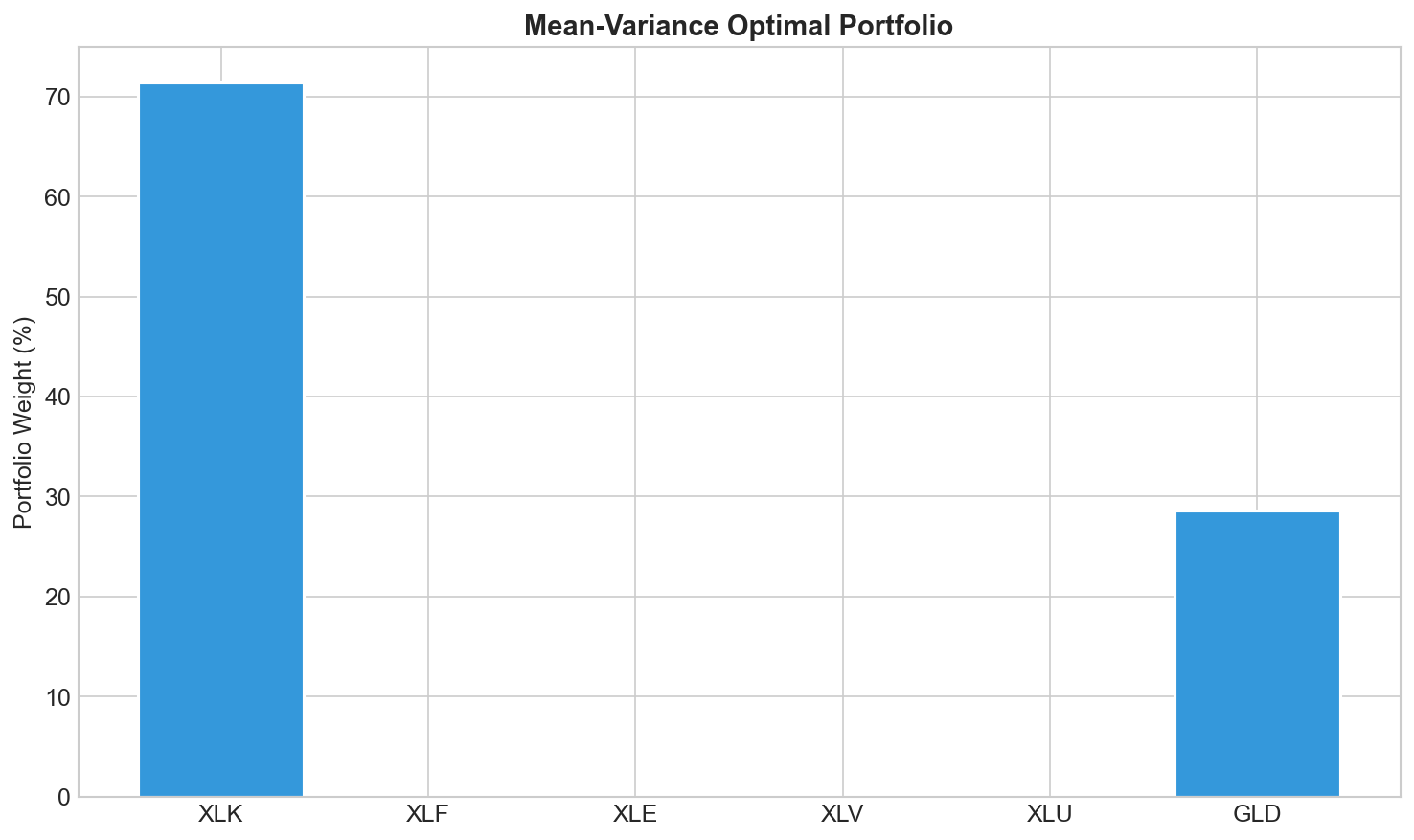
Heavy allocation to XLK (Technology) and GLD (Gold). XLK had strong returns in this period. GLD helps because its low correlation with everything else brings down portfolio variance without hurting returns much.
The Problem with Variance
MV treats upside and downside volatility the same. A 5% gain and a 5% loss both add to variance equally.
But that’s not how people experience risk. Losses sting more than gains feel good. And real returns aren’t symmetric. Big drops happen more often than big rallies. The distribution has a fat left tail.
Two statistics capture what variance misses:
Skewness measures asymmetry. You take each return’s deviation from the mean, cube it, average those cubes, and divide by standard deviation cubed.
Positive skewness: longer right tail, occasional big gains
Negative skewness: longer left tail, occasional big losses
Zero: symmetric
Most stocks have negative skewness. Crashes are more common than melt-ups.
Kurtosis measures how fat the tails are. Same idea but raise deviations to the fourth power instead of the third. Subtract 3 so a normal distribution scores zero.
Positive kurtosis: fat tails, extreme events happen more than you’d expect
Negative kurtosis: thin tails, extreme events are rare
Zero: normal distribution
Most stocks have positive kurtosis. The 2008 crash and COVID’s March 2020 drop were supposedly “six sigma” events. Once in a million years stuff. Except they happen way more often than that.
MVSK Optimization
MVSK extends the utility function:
U = μ - (λ/2)σ² + (λₛ/6)S - (λₖ/24)K
Where:
S is portfolio skewness. We reward positive values (more upside surprises).
K is portfolio kurtosis. We penalize positive values (fewer extreme events).
λₛ and λₖ control how much we care about each.
The 1/6 and 1/24 coefficients come from Taylor series math. The signs make sense: add skewness (we like it positive), subtract kurtosis (we want it low).
How do MVSK weights compare to MV?
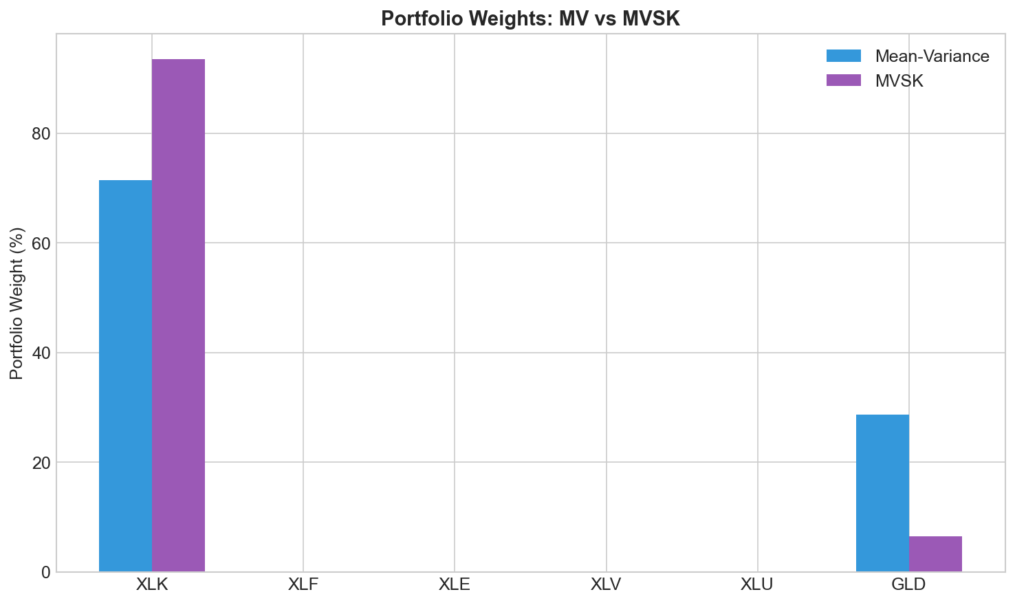
Often the differences are subtle. MVSK might shift weight toward assets with better skewness even if they’re slightly more volatile. Trading variance for better tail behavior.
Out-of-Sample Test
Optimizing on historical data is easy. Does it work on data the optimizer never saw?
We trained on 2018-2021 and tested on 2021-2024. Here’s how $1 grows under each strategy:
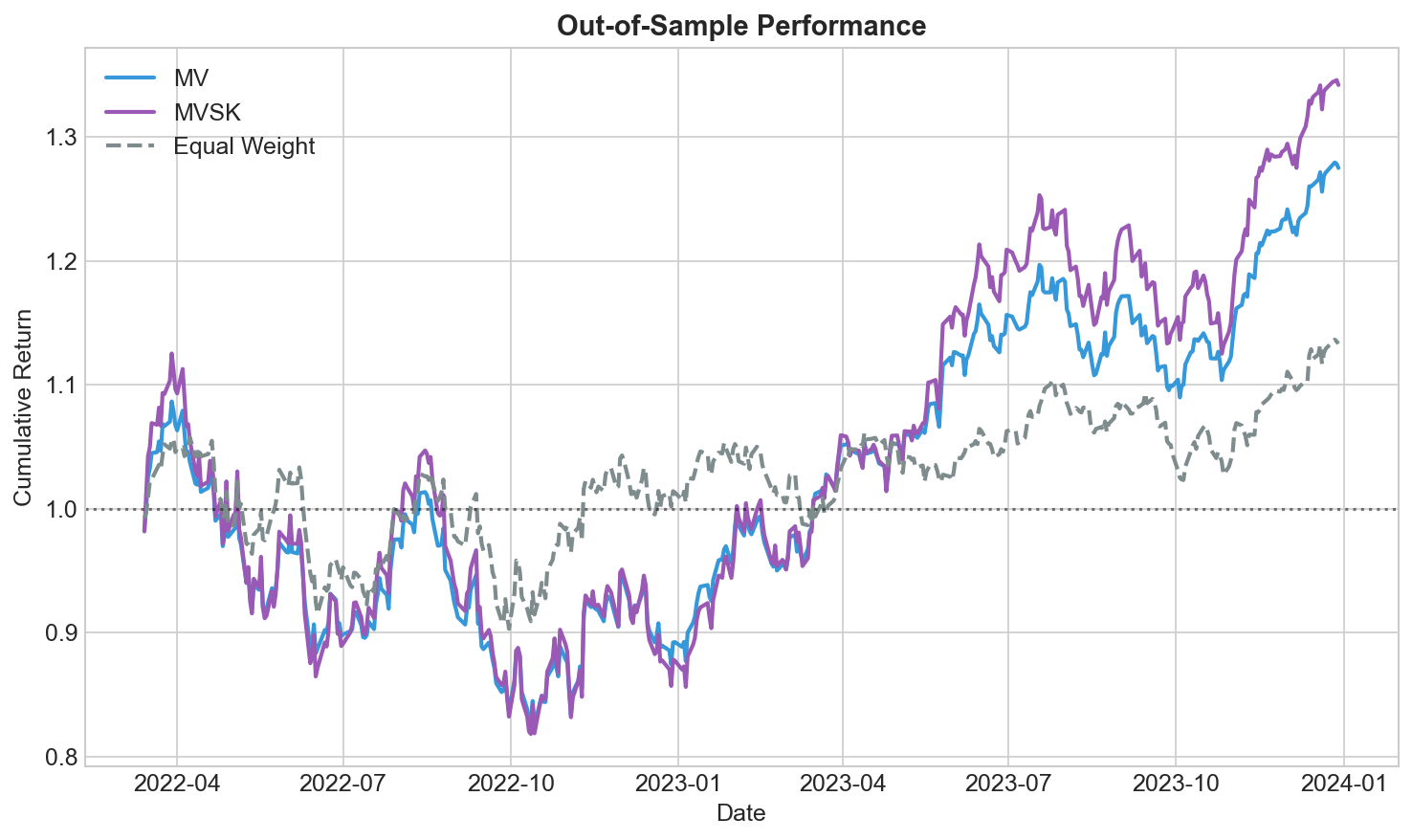
During calm markets, they track closely. During rough patches like late 2022, differences emerge. Neither dominates everywhere.
The return distributions:
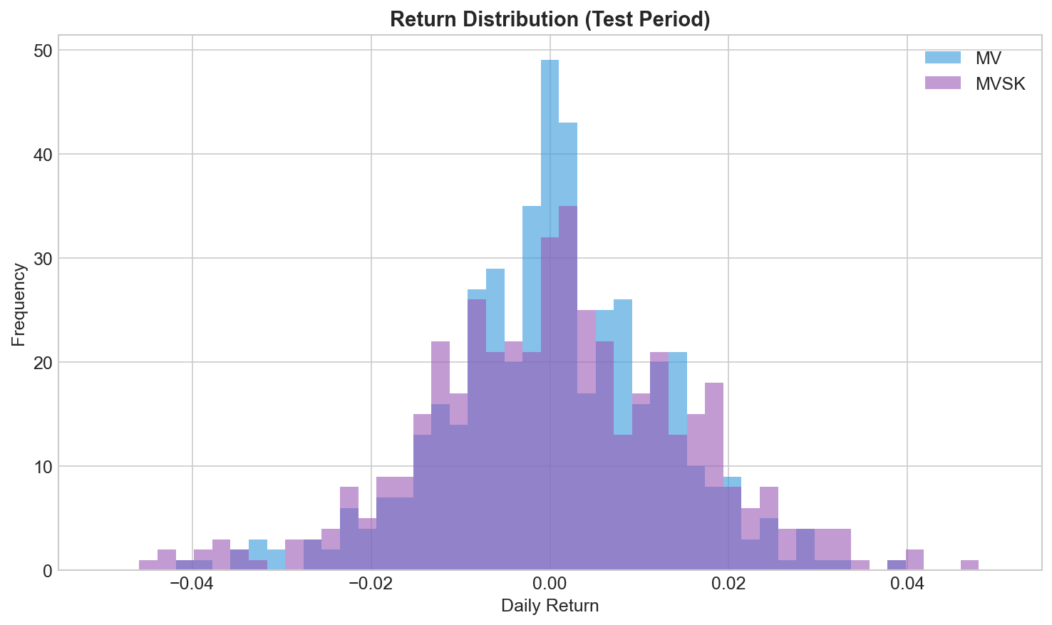
Similar centers, but different tails. That’s where MVSK focuses.
How Risk Aversion Changes Everything
λ matters a lot. Here’s how weights shift as you crank it up:
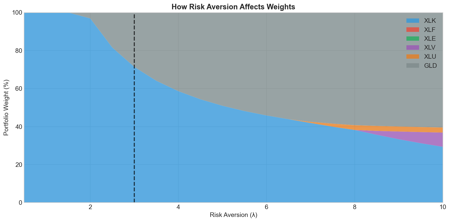
Low λ (aggressive): pile into XLK for returns. High λ (conservative): shift toward XLU and GLD for stability.
The vertical line is λ = 3. Balanced, not too hot, not too cold.
Summary
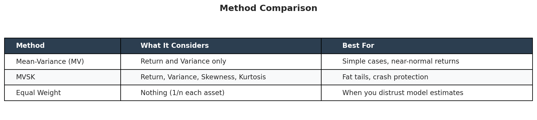
What to remember:
MV is the default for a reason. Simple, well understood, works fine when returns are roughly normal. Start here.
MVSK adds tail awareness. Worried about crashes? MVSK penalizes bad skewness and fat tails. Costs you some complexity.
Don’t sleep on equal weight. Zero estimation error. When your estimates are garbage (often true), equal weight beats fancy optimizers out of sample.
Always test out of sample. Any optimizer looks good on its training data. Reserve a holdout period.
λ controls the aggression. Start around 3, adjust to taste.