
Risky Business: Beginner's guide to measuring portfolio risk
A simple look at understanding risk metrics

When you’re investing your money, you’re goal is very simple. Make the most money. Suppose you’re deciding between two portfolios with the following 5 year returns. Which would you invest in?
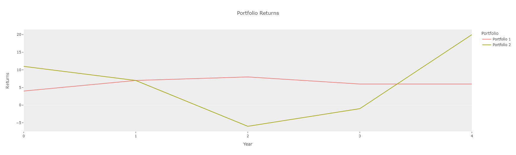
Now they both have the same average return of 6.2% and similar annualized returns of 7.4% and 7.1% respectively. In addition to returns, we also want to factor in risk in our decision making. Notice portfolio 2 is more volatile. Imagine you’re saving up to buy a house in a couple years, you might have a lower risk tolerance given that you need the money sooner. Versus a retirement account you would be open to more risk. This is where we need a way to quantify the risk
Sharpe Ratio
The most common way to measure risk in a portfolio is the sharpe ratio.
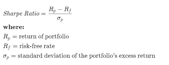
Decomposing this, we are simply looking at the ratio of the excess returns vs its risk, where the risk is we measure as the standard deviation of returns. I.E, getting more bang for my buck. For each unit of risk, I want more return.
Now we use a risk free rate as a baseline to calculate the “excess return”. One can invest in treasury bill which are generally risk free to serve as a baseline as if you are going to be taking some risk, you want it have better returns than the baseline.
def get_sharpe_ratio(returns, annual_risk_free_rate=0.05):
    """
    Determines the Sharpe ratio of a strategy.

    Parameters
    ----------
    returns : pd.Series or np.ndarray
        Daily returns of the strategy, noncumulative.
    adjustment_factor : int, float
        Constant daily benchmark return throughout the period.
    Returns
    -------
    sharpe_ratio : float
    Note
    -----
    See https://en.wikipedia.org/wiki/Sharpe_ratio for more details.
    """
    daily_risk_free_rate = (1 + annual_risk_free_rate) ** (1 / 252) - 1
    returns_risk_adj = returns - daily_risk_free_rate
    excess_returns = returns.mean()-daily_risk_free_rate
    volatility = returns.std()
    return np.sqrt(252)*excess_returns/volatility #annaulize it
Sortino Ratio
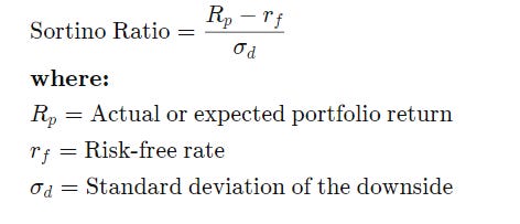
In addition, we can look at the Sortino Ratio. Notice the formula is the exact same, excess this time we only look at the standard deviation of the downside. AKA, we only focus in the negative returns. Since we’re focusing on the negative returns, this will inform us about worrying about the big losses in the portfolio. Yes we can have positive volatility, but that’s still positive returns so in this case I am comfortable with that volatility vs swings in the other direction.
def get_sortino_ratio(returns, annual_risk_free_rate=0.05):
    """
    Determines the Sharpe ratio of a strategy.

    Parameters
    ----------
    returns : pd.Series or np.ndarray
        Daily returns of the strategy, noncumulative.
    adjustment_factor : int, float
        Constant daily benchmark return throughout the period.
    Returns
    -------
    sharpe_ratio : float
    Note
    -----
    See https://en.wikipedia.org/wiki/Sharpe_ratio for more details.
    """
    daily_risk_free_rate = (1 + annual_risk_free_rate) ** (1 / 252) - 1
    returns_risk_adj = returns - daily_risk_free_rate
    excess_returns = returns.mean()-daily_risk_free_rate
    negative_volatility = returns_risk_adj[returns_risk_adj<0].std()
    return np.sqrt(252)*excess_returns/negative_volatility  #Annualize it
Putting it all together
We usually have to deal with much more nuanced data than a 5 year return. But the beauty of this is all we need is returns data to calculate the ratio. Suppose I’m deciding in portfolios in just pure Tesla Stock or pure Apple stock. I see that the daily returns for the past 5 years below, which is ugly to look. So let’s just feed in the daily returns to measure our risk
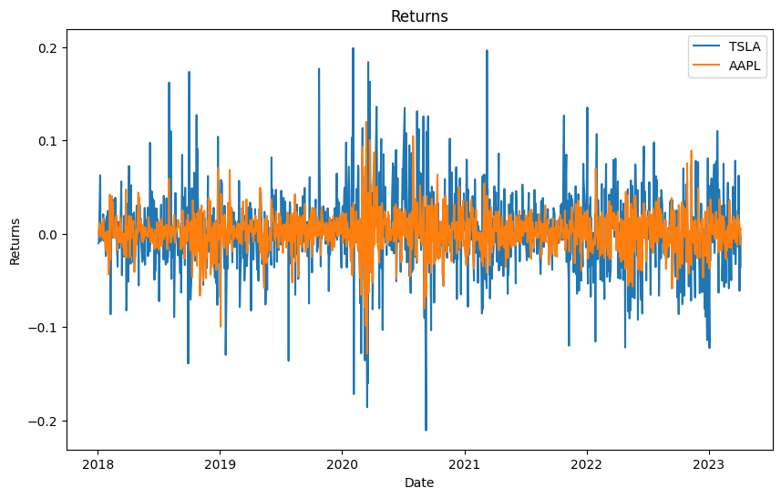
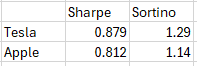
We can observe that TSLA gives us a better Sharpe & Sortino Ratio than apple. In practice, we deal with large portfolios with varying stocks and weights. However it’s really just plug and play. I just need the returns of the portfolios, I don’t care about the compositions.